Sampling distributions

Options for finding the sampling distribution:

• Derive it mathematically
• Can’t derive the distribution?
  • Derive properties of the distribution
  • Simulate
  • Approximate

Normal population: set up

Population distribution: \(Y \sim N(\mu, \sigma^2)\)

Sample: \(Y_1, \ldots, Y_n\) i.i.d from population

Sample statistic: Sample mean = \(\overline{Y} = \frac{1}{n}\sum_{i=1}^n Y_i\)

What is the sampling distribution of the sample mean?

Normal population: derivation

\(Y_1 + Y_2 \sim\)

\(Y_1 + Y_2 + Y_3 \sim\)

\(Y_1 + Y_2 + \ldots + Y_n \sim\)

\(\overline{Y} = \frac{Y_1 + Y_2 + \ldots + Y_n}{n} \sim\)

Bernoulli population

Population distribution: \(Y \sim \textit{Bernoulli}(p)\)

E.g US voters where \[ Y = \begin{cases} 1, & \text{Supports single payer health care} \\ 0, & \text{Does not support single payer health care} \end{cases} \]

Sample: \(Y_1, \ldots, Y_n\), i.i.d from population

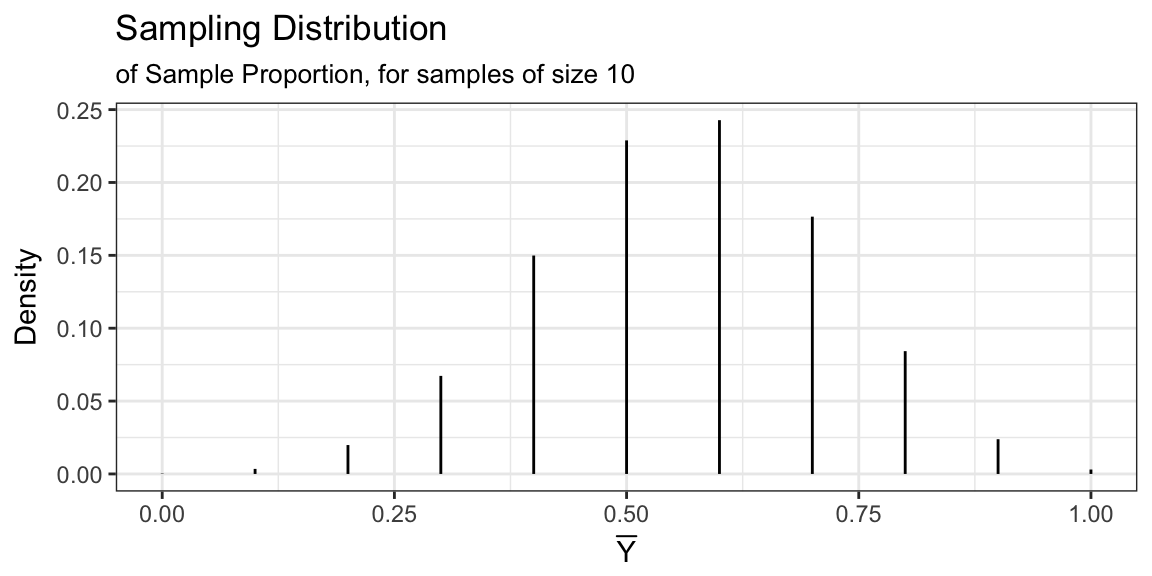
Sample Statistic: Sample mean = \(\overline{Y} = \frac{1}{n}\sum_{i=1}^n Y_i =\) gives the sample proportion

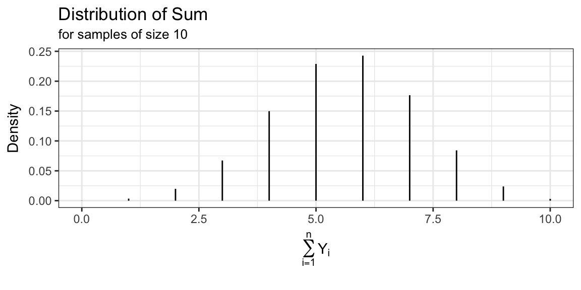
What is the sampling distribution of the sample proportion? \(\sum_{i=1}^n Y_i \sim \text{Binomial} (n, p)\)

Bernoulli population

E.g. \(p = 0.56\), \(n = 10\)

Bernoulli population

E.g. \(p = 0.56\), \(n = 10\)

Can’t derive in these situations

• Population: \(Y \sim Uniform(a, b)\)
• Sample: size \(n\) i.i.d
• Statistic: sample mean or sample variance
• No closed form solution

• Population \(Y \sim\) unknown
• Sample: size \(n\) i.i.d
• Statistic: anything
• Can’t derive because we don’t know population distribution

What to do?

1. Derive parameters of sampling distribution
2. Simulate the sampling distribution
3. Approximate the sampling distribution

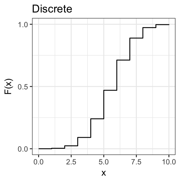
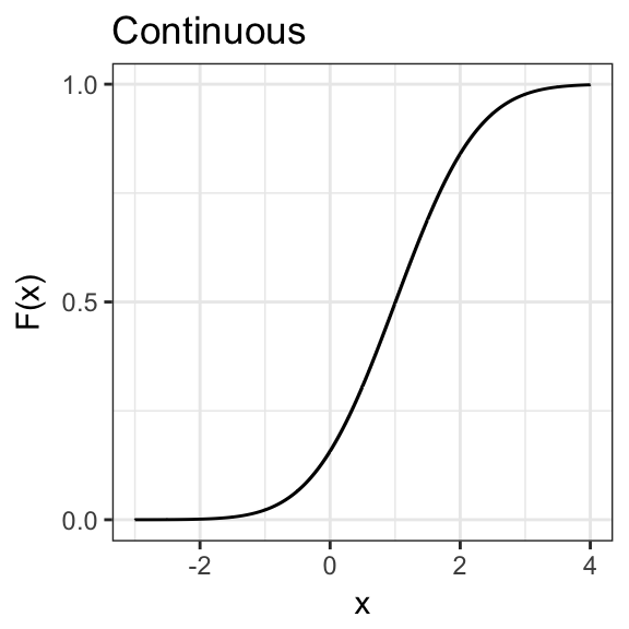
Cumulative Density Function

The cumulative density function of a random variable \(X\) is \[ F(x) = P(X \le x) \]

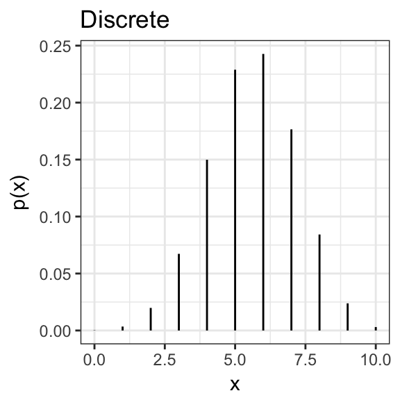
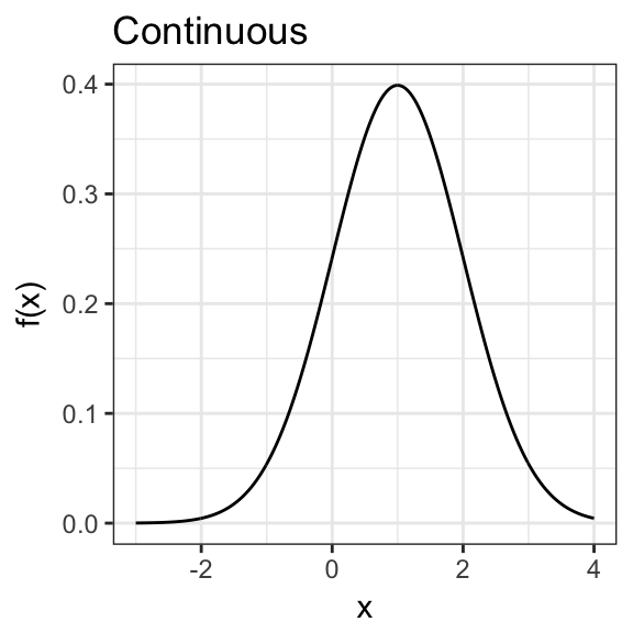
Probabilty Density/Mass Function

For continuous distributions we can define the probability density function:

\[ f(x) = \frac{d}{dx}F(x) \approx \frac{P\left(X \in (x - \Delta,\, x + \Delta) \right)}{2\Delta} \] For discrete distributions we have probability mass function:

\[ p(x) = P(X = x) \]

Probabilty Density/Mass Function

Expectation (Mean)

The expectation (or mean) of a random variable, \(X\), is

\[ \begin{aligned} E(X) &= \int\limits_{-\infty}^{\infty}xf(x) dx \quad &\text{for continuous distributions}\\ E(X) &= \sum\limits_{x: p(x) > 0} x p(x) \quad &\text{for discrete distributions} \end{aligned} \]

Expectation Properties

For any random variables \(X\) and \(Y\) (don’t need independence)

\(E(X + Y) = E(X) + E(Y)\)

\(E(a_1X_1 + \ldots + a_nX_n) = a_1E(X_1) + \ldots + a_nE(X_n)\)

Known as the linearity property.

Variance and Covariance

The variance of r.v. \(X\) is \[ Var(X) = E\bigl[ \left(X - E(X)\right)^2 \bigr] = E[X^2] - \left(E[X]\right)^2 \]

The covariance between r.v.’s \(X\) and \(Y\) is \[ Cov(X, Y) = E\left[\bigl(X- E(X) \bigr)\bigl(Y - E(Y) \bigr)\right] \] If \(X\) and \(Y\) are independent \(Cov(X, Y) = 0\) (converse isn’t true)

\(Cov(X, X) = Var(X)\)

Variance Properties

For any random variables \(X\) and \(Y\) (don’t need independence)

\(Var(X + Y) = Var(X) + Var(Y) + 2Cov(X, Y)\)

\(Var(X - Y) = Var(X) + Var(Y) - 2Cov(X, Y)\)

For random variables \(X_1, \ldots, X_n\) \[ \begin{aligned} \textit{Var}& \left(a_1 X_1 + \ldots + a_n X_n \right)= a_1^2 \textit{Var}(X_1) + \ldots + a_n^2 \textit{Var}(X_n) \, +\\ & a_1a_2 \textit{Cov}(X_1, X_2) + a_1a_3\textit{Cov}(X_1, X_3) + \ldots + a_1a_n\textit{Cov}(X_1, X_n) \, + \\ & \vdots \\ & a_na_1\textit{Cov}(X_n, X_1) + a_na_2\textit{Cov}(X_n, X_2) + \ldots + a_na_{n-1}\textit{Cov}(X_n, X_{n-1}) \end{aligned} \]

Next time…

Use these properties to derive mean and variance for sampling distributions.