Deriving Properties of the Sampling Distibution
Given a specific statistic it’s sometimes possible to derive properties of its sampling disitbrution without knowing the population distribution shape.
I.e. apply properties of expectation and variance to derive expectation and varinace of sampling distribution.
Unknown population distribution
Imagine we don’t know the population distribution, but we do know it has mean, \(\mu\), and variance \(\sigma^2\)
Population: \(\sim (\mu, \sigma^2)\)
Sample: \(n\) i.i.d from population
Sample statistic: Sample mean
Expectation of sampling distribution of sample mean
\(E(\frac{1}{n}(Y_1 + Y_2 + \ldots + Y_n))\) =
The sampling distribution of the sample mean is centered around the population mean.
Variance of sampling distribution of sample mean
\(Var(\frac{1}{n}(Y_1 + Y_2 + \ldots + Y_n))\) =
The variance of the sampling distribution of the sample mean is smaller than the population variance (\(n > 1\)), and decrease with increasing \(n\).
More properties of sample means
Weak Law of Large Numbers (WLLN)
For i.i.d samples from a population with mean \(\mu\):
As the sample size increases to infinity (\(n \rightarrow \infty\)), the sample mean converges in probability to the population mean, \(\mu\).
Probability of sample mean being some small distance from \(\mu\) goes to zero as sample size increases
We write: \[ \overline{Y} \rightarrow_p \mu \]
Simulating Sampling Distributions
Simulating Sampling Distributions
Just knowing mean and variance of the sampling distribution isn’t generally enough.
If we know or hypothesize a population distribution we can simulate to obtain the sampling distribution for any statistic.
Simulation Set Up
Specify a known or hypothesized population distribution.
Repeat \(B\) times:
- Draw sample of size \(n\) from the population distribution
- Calculate the desired sample statistic from the sample
- Record the value of sample statistic
Get \(B\) sample statistics (from \(B\) samples)
For large \(B\), the distribution of the \(B\) sample statistics approximates the true sampling distribution. Why?
Your Turn
Let \(X\) be a random variable with an unknown distribution.
I obtain \(X_1, \ldots, X_{10}\) i.i.d samples from the distribution. I get:
5, 3, 7, 4, 4, 3, 7, 2, 7, 3
How would you estimate \(P(X \le 5)\)?
Empirical Distribution Function
The empirical cumulative distribution function (ECDF) for a sample \(X_1, \ldots, X_n\) is:
\[ \widehat{F}(x) = \frac{1}{n}\sum_{i = 1}^n \pmb{1}\left\{ X_i \le x \right\} \]
Intuition: the ECDF at \(x\), is the sample proportion of observed values less than or equal to \(x\).
Empirical Distribution Function
\(\widehat{F}(x)\) is a sample mean of the random variable \(\pmb{1}\left\{ X_i \le x \right\}\) therefore the Weak Law of Large Numbers applies.
\(E\left[\pmb{1}\left\{ X_i \le x \right\}\right] = F(x)\)
\(\widehat{F}(x) \rightarrow_p F(x)\)
So, the ECDF converges to the true cumulative distribution function.
In practice this means we can use our simulated values to approximate the distribution of the sampling distribution.
Example: Commute times
Population: ST551 students present on first day of class Fall 2017 Variable of interest: Commute time in minutes
Parameter: Population mean
What’s the sampling distribution for the sample mean of samples of size 5?
What’s the probability the sample mean from a sample of size 5 is less than 10 minutes?
Example: Commute times
Specify a known or hypothesized population distribution.
Repeat \(B\) times:
- Draw sample of size \(n\) from the population distribution
- Calculate the desired sample statistic from the sample
- Record the value of sample statistic
Get \(B\) sample statistics (from \(B\) samples)
Example: Commute times
Population: all commute times from index cards
Repeat \(B\) times:
- Draw 5 cards at random
- Find mean commute time of sample
- Record the value
Get \(B\) sample statistics (from \(B\) samples)
Example: Commute times
Population: class_data$commute_times
Repeat n_sim times:
one_sample <- sample(class_data$commute_times, size = 5)mean(one_sample)- Record
mean(one_sample)
Example: Commute times
library(tidyverse)
n <- 5
n_sim <- 1000

# Generate many samples
samples <- rerun(.n = n_sim,
  sample(class_data$commute_time, size = n))

# Do something to each sample
sample_means <- map_dbl(samples, ~ mean(.x))
Example: Commute times
Examining the distribution of the simulated sample statistics
# Sampling dist. histogram
ggplot() +
  geom_histogram(aes(x = sample_means), binwidth = 1) +
  theme_bw() +
  labs(x = "Sample mean commute time",
    title = "Sampling Distribution",
    subtitle = "for sample mean and sample size, n = 5")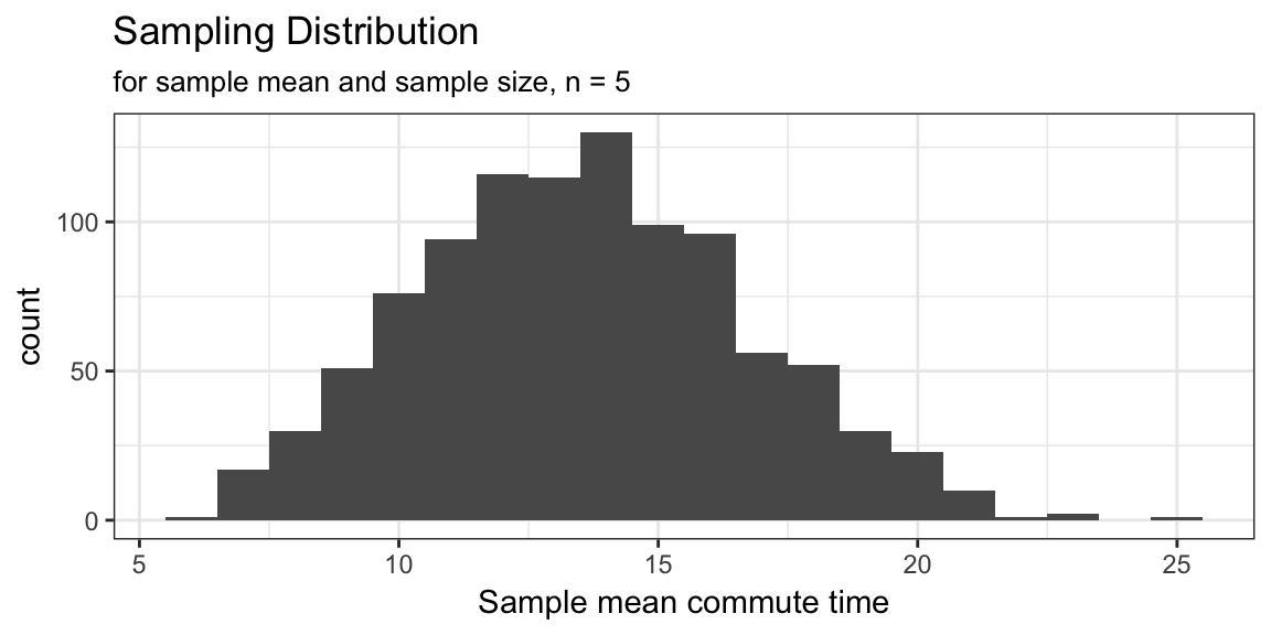
Example: Commute times
Using the simulated sample means to estimate a probability.
What’s the probability the sample mean from a sample of size 5 is less than 10 minutes?
# Estimate a specific probability
mean(sample_means < 10)
## [1] 0.129Can’t I just write a for loop?
Yes, you could write a for loop. I almost never do anymore, because a functional style results in lots less book keeping and code that more clearly expresses the intent rather than the implementation.
In general:
There are lot’s of ways to get anything done in R.
I’ll show you one way (that comes from a lot of experience and recent innovations).
You don’t have to use my way.
You should always aim for code that: 1. Is correct 2. Is clear (i.e. understandable to a fellow human being)
Approximate Sampling Distribution
Central Limit Theorem (CLT)
If the population distribution of a variable \(X\) has population mean \(\mu\) and (finite) population variance \(\sigma^2\), then the sampling distribution of the sample mean becomes closer and closer to a Normal distribution as the sample size n increases.
We can write: \[ \overline{X} \, \dot \sim \, N\left(\mu, \frac{\sigma^2}{n}\right) \] for large values of \(n\), where the symbol \(\dot \sim\) means approximately distributed as.