Inference for a population mean

What do we do if we don’t know \(\sigma^2\)? Realistically this is always the case

We can estimate \(\sigma^2\), just like we estimated \(\mu\):

• We used the sample mean to estimate the population mean
• We can use the sample variance to estimate the population variance

Sample variance

The sample variance for a sample \(Y_1, \ldots, Y_n\) is: \[ s^2 = \frac{1}{n-1}\sum_{i=1}^n \left(Y_i - \overline{Y}\right)^2 \]

Facts about the sampling distribution of the sample variance:

• The mean is \(\sigma^2\), i.e. \(s^2\) is an unbiased estimate of \(\sigma^2\)
• As the sample size \(n\) gets larger, \(s^2\) gets closer and closer to the true population variance \(\sigma^2\), i.e. \(s^2\) is consistent estimate of \(\sigma^2\)

t-statistic

If we replace \(\sigma^2\) with \(s^2\) in the Z-statistic for testing \(H_0: \mu = \mu_0\), we get a t-statistic:

\[ Z(\mu_0) = \frac{\overline{Y} - \mu_0}{\sqrt{\sigma^2/n}} \rightarrow t(\mu_0) = \frac{\overline{Y} - \mu_0}{\sqrt{s^2/n}} \]

Reference distribution

We compared the Z-statistic to N\((0, 1)\)

• Why? N\((0, 1)\) is the distribution we expect for \(Z\), when the null hypothesis is true

What should we compare a t-statistic to?

• \(s^2\) will sometimes be smaller than \(\sigma^2\), sometimes bigger
• Introduces additional variability into our test statistic

t-distribution

The null distribution for a t-statistic is the t-distribution.

the t-distribution is a family of distributions defined by a single parameter the degrees of freedom

Notation:

• \(t_(1)\) - t-distribution with 1 degree of freedom
• \(t_(3)\) - t-distribution with 3 degrees of freedom
• \(t_(v)\) - t-distribution with \(v\) degree of freedom

Looks a lot like a Standard normal but with heavier tails and sharper peak.

t-distribution

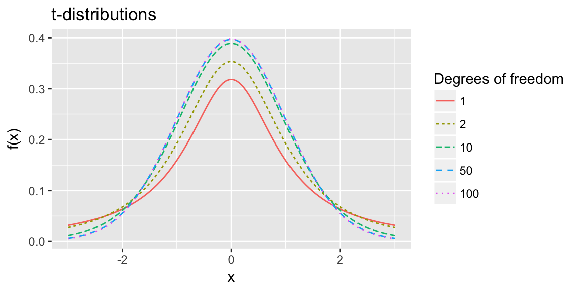
As \(v \rightarrow \infty\) \(t_{(v)}\) approaches the Standard Normal density.

t-test: Inference for population mean

• If the population is exactly Normal:

  • \(\overline{Y}\) exactly Normal.
  • t-statistic is exactly a t-distribution with \(n-1\) degrees of freedom

• If population is anything with finite variance:

  • \(\overline{Y}\) approximately Normal,
  • t-statistic approximately t-distribution with \(n-1\) d.f.

t-test: Inference for population mean

Rather than coming from a Standard Normal:

• Rejection region critical values come from t-distribution quantiles
• CI multipliers come from t-distribution quantiles
• P-values come from the cumulative distribution function of the t-distribution

In R: pt(q, df), qt(p, df), dt(x, df)

t-test: Summary

Data Setting One sample, no explanatory variable \(Y_1, \ldots, Y_n\) i.i.d from population with unknown variance \(\sigma^2\)

Null hypothesis \(H_0: \mu = \mu_0\)

Test statistic \[ t(\mu_0) = \frac{\overline{Y} - \mu_0}{\sqrt{s^2/n}} \]

Reference distribution \(t(\mu_0) \dot \sim t_{(n-1)}\)

t-test: Summary

Rejection Region for level \(\alpha\) test

One sided \(H_A: \mu < \mu_0\)	Two sided \(H_A: \mu \ne \mu_0\)	One sided \(H_A: \mu > \mu_0\)
\(t(\mu_0) < t_{(n-1)\alpha}\)	\(|t(\mu_0)| > t_{(n-1)1-\alpha/2}\)	\(t(\mu_0) > t_{(n-1)1 - \alpha}\)

\(t_{(n-1) \alpha}\) = qt(alpha, df = n - 1)

t-test: Summary

p-values given an observed \(t(\mu_0) = t\)

One sided \(H_A: \mu < \mu_0\)	Two sided \(H_A: \mu \ne \mu_0\)	One sided \(H_A: \mu > \mu_0\)
\(F_t(t; n-1)\)	\(2\left(1 - F_t(|t|; n-1)\right)\)	\(1 - F_t(t; n-1)\)

\(F_t(t; n-1)\) = pt(t, df = n-1)

Confidence Intervals \((1-\alpha)100\%\)

\[ \left( \overline{Y} - t_{(n-1)1 - \alpha/2} \, \sqrt{\frac{s^2}{n}}, \, \overline{Y} + t_{(n-1)1 - \alpha/2} \, \sqrt{\frac{s^2}{n}} \right) \]

Standard error

\[ Var(\overline{Y}) = \frac{\sigma^2 }{n} \] We estimated \(\sigma^2\) with \(s^2\), hence estimate \(Var(\overline{Y})\) with

\[ \widehat{Var}(\overline{Y}) = \frac{s^2}{n} \]

Square root of this, often called, standard error of the mean:

\[ \text{SE}(\overline{Y}) = \frac{s}{\sqrt{n}} \]

In general standard error refers to the estimated standard deviation of an estimator.

Next time

Population proportions (a special case of population means)