Exact Binomial Test: Takeaways

“Exact” because it uses the exact sampling distribution of the sum of \(Y_i\).

The actual Type I error rate will never be more than \(\alpha\), but may be substantially less (i.e. conservative).

You can invert the test to get a confidence interval, but there isn’t an easy closed form for the interval.

Exact Binomial Test: In R

binom.test(x = 7, n = 12, p = 0.4)

## 
##  Exact binomial test
## 
## data:  7 and 12
## number of successes = 7, number of trials = 12, p-value = 0.2417
## alternative hypothesis: true probability of success is not equal to 0.4
## 95 percent confidence interval:
##  0.2766697 0.8483478
## sample estimates:
## probability of success 
##              0.5833333

Exact Binomial Test: In R

binom.test(x = 7, n = 12, p = 0.4)

x - count of 1’s, i.e. \(\sum_{i=1}^{n}Y_i\)
n - sample size
p - \(p_0\), the hypothesized population proportion

The reported CI is a Clopper-Pearson confidence interval, based on the exact distribution but with equal tails (i.e. try to get \(\alpha/2\) in each tail).

Approximate Binomial Test

Use fact that: \[ \overline{Y} \dot\sim N\left( E(Y) , \frac{Var(Y)}{n}\right) = N\left( p , \frac{p(1-p)}{n}\right) \]

Leads to the Z-test where:

\[ Z(p_0) = \frac{\hat{p} - p_0}{\sqrt{p_0 (1 - p_0)/n}} \] \(\hat{p} = \overline{Y}\) = sample proportion

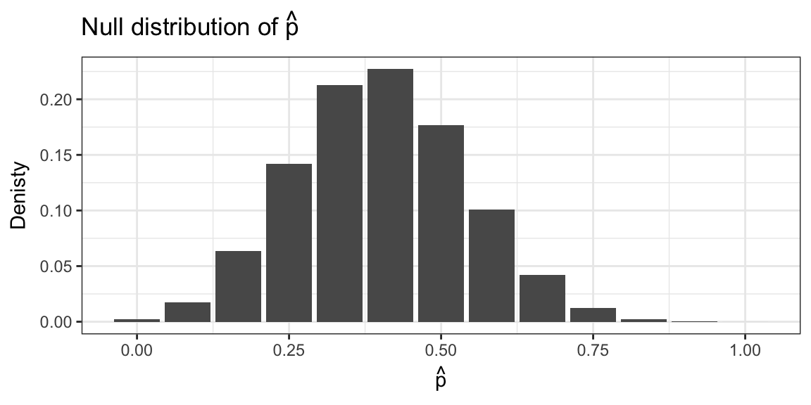
Exact distribution of sample proportion

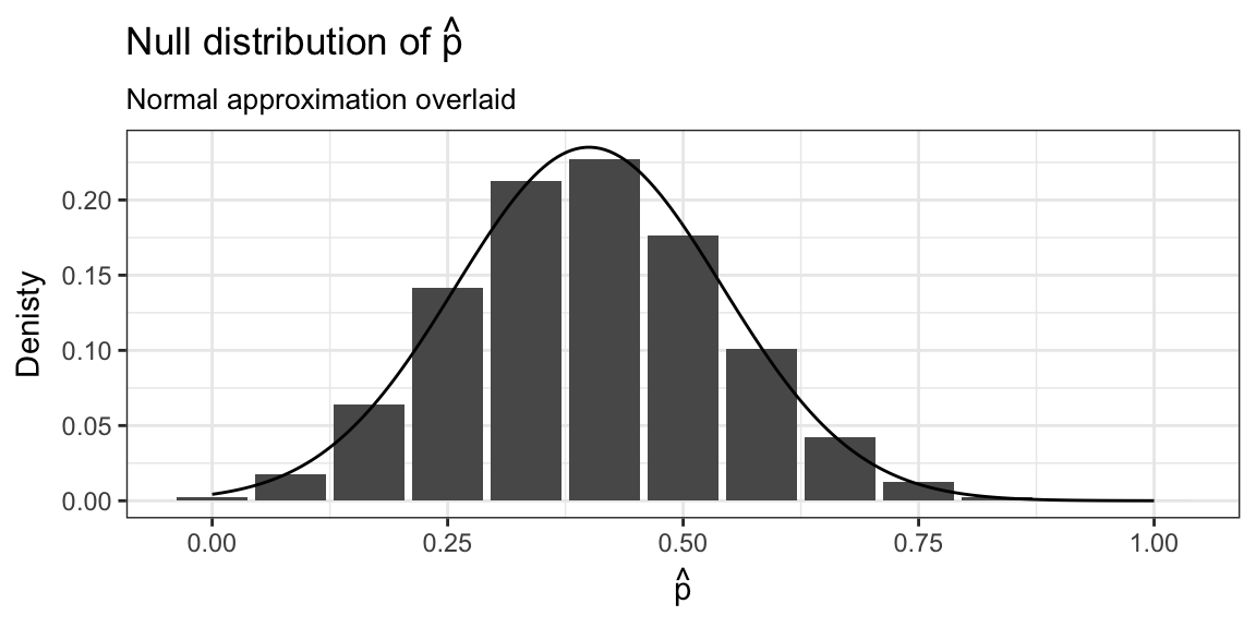
Approximate distribution of sample proportion

Your turn

library(openintro)
census %>% 
  group_by(sex) %>%
  summarise(n = n())

## # A tibble: 2 x 2
##      sex     n
##   <fctr> <int>
## 1 Female   232
## 2   Male   268

Find:

1. \(\hat{p}\)

2. The Z-statistic, for the test of \(H_0: p = 0.5\)

Your turn

A confidence interval?

Need to invert test, i.e. find all \(p_0\) such that: \[ |Z(p_0)| = \left| \frac{\hat{p} - p_0}{\sqrt{p_0 (1 - p_0)/n}}\right| > z_{1-\alpha/2} \]

It’s hard…

Instead use:

\[ \hat{p} \pm z_{1-\alpha_2} \sqrt{\frac{\hat{p}(1-\hat{p})}{n}} \] Based on inverting a (Wald) test with statistic:

\[ Z_w(p_0) = \frac{\hat{p} - p_0}{\sqrt{\hat{p} (1 - \hat{p})/n}} \]

Asymptotically equivalent to \(Z(p_0)\) (happens to be the Score test)

Your turn

library(openintro)
census %>% 
  group_by(sex) %>%
  summarise(n = n())

## # A tibble: 2 x 2
##      sex     n
##   <fctr> <int>
## 1 Female   232
## 2   Male   268

Find:

1. 95% CI for \(p\).

Can lead to contradictions

A score test, \(Z(p_0)\), might not agree with a Wald interval.

Learn to live with it…or don’t calculate things by hand.

In R

prop.test(x = 232, n = 232 + 268, p = 0.5, correct = FALSE)

## 
##  1-sample proportions test without continuity correction
## 
## data:  232 out of 232 + 268, null probability 0.5
## X-squared = 2.592, df = 1, p-value = 0.1074
## alternative hypothesis: true p is not equal to 0.5
## 95 percent confidence interval:
##  0.4207282 0.5078208
## sample estimates:
##     p 
## 0.464

In R

prop.test(x = 232, n = 232 + 268, p = 0.5, correct = FALSE)

Equivalent to \(Z(p_0)\) and inverts to get confidence interval (i.e. p-value and CI will agree).

Reports X-squared, \(\chi^2\) statistic, take square root to get \(Z\)

When to use the Approximate Binomial test?

Compare to:

binom.test(x = 232, n = 232 + 268, p = 0.5)

## 
##  Exact binomial test
## 
## data:  232 and 232 + 268
## number of successes = 232, number of trials = 500, p-value =
## 0.1174
## alternative hypothesis: true probability of success is not equal to 0.5
## 95 percent confidence interval:
##  0.4196128 0.5088153
## sample estimates:
## probability of success 
##                  0.464

When to use the Approximate Binomial test?

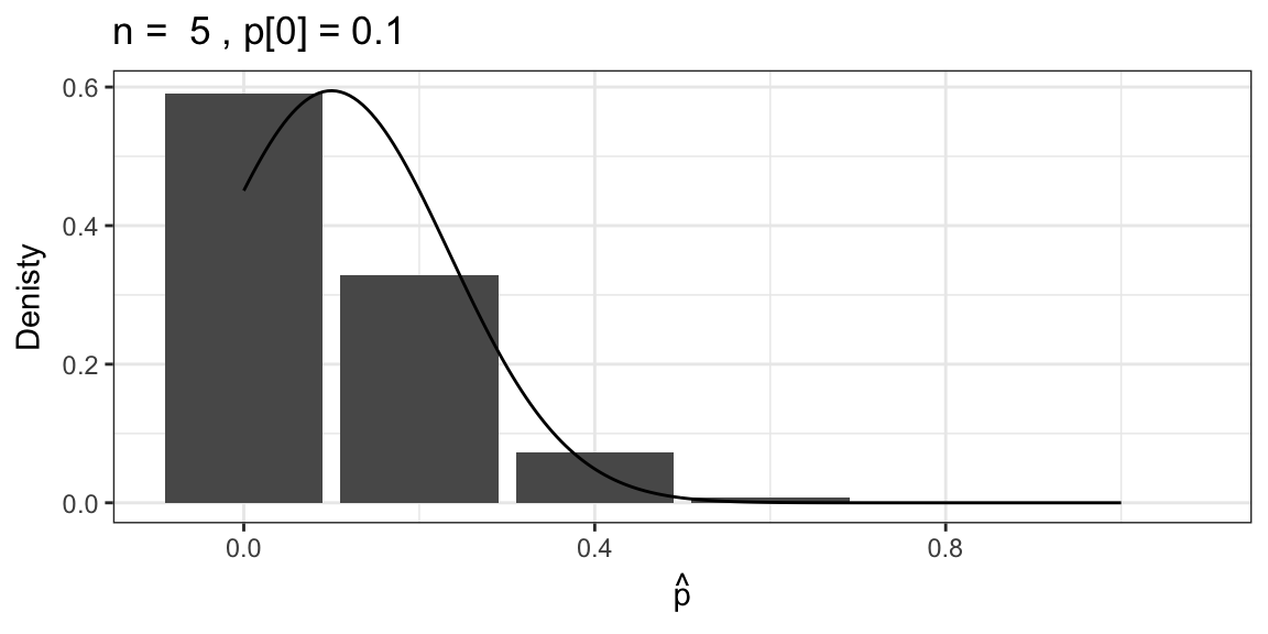
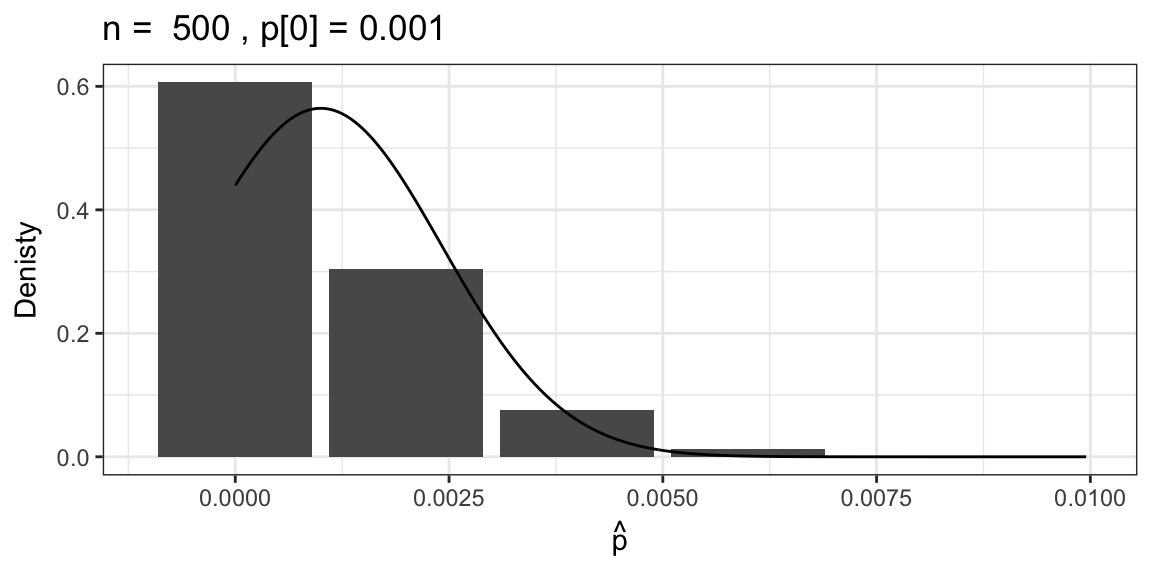
The approximation isn’t great for small expected counts.

OK to use the approximation if: \(np_0 > 5\) and \(n(1-p_0)> 5\)

(Or something similar)

Next time…

Use Binomial test as a way to look at population median.