Kolmogorov-Smirnov Test

Population: \(Y \sim\) some population distribution with c.d.f \(F\)

Sample: n i.i.d from population, \(Y_1, \ldots, Y_n\)

Parameter: Whole CDF

Null hypothesis: \(H_0: F = F_0\), versus \(H_A: F \ne F_0\)

Kolmogorov-Smirnov Test

Test statistic

\[ D(F_0) = \sup_{y} \left| \hat{F}(y) - F_0(y) \right| \]

where \(\hat{F}(y)\) is the empirical cumulative distribution function:

\[ \hat{F}(y) = \frac{1}{n}\sum_{i= 1}^{n} \pmb{1}\left\{ Y_i \le y \right\} \]

and \(F_0\) is the cumulative distribution function for the null hypothesized distribution.

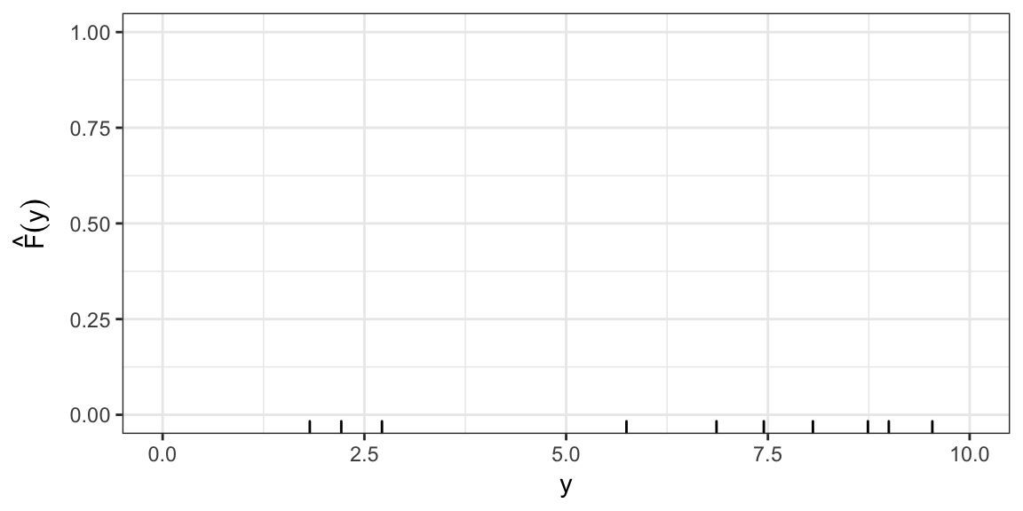
ECDF: Example

Sample values: 1.8, 2.2, 2.7, 5.7, 6.9, 7.4, 8.1, 8.7, 9 and 9.5

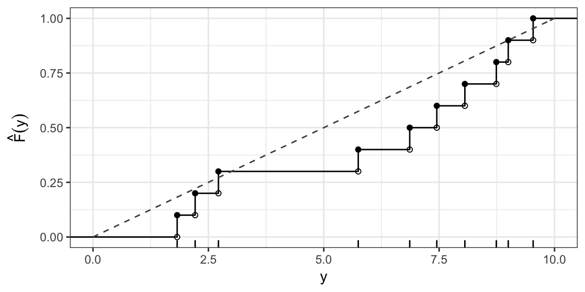
KS test statistic: Uniform(0, 10)

Say, \[ H_0: F(Y) = \begin{cases} 0, & y \le 0 \\ \frac{y}{10}, & 0 < y \le 10 \\ 1, & y > 10 \end{cases} \]

I.e. \(H_0: Y \sim \text{Uniform}(0, 10)\)

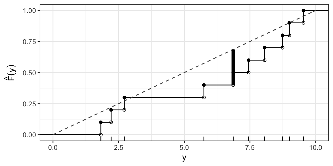
KS test statistic: Uniform(0, 10) cont.

\(D(F_0) = \sup_{y} \left| \hat{F}(y) - F_0(y) \right| \approx 0.29\) (occurs at \(y\) just less than 6.9)

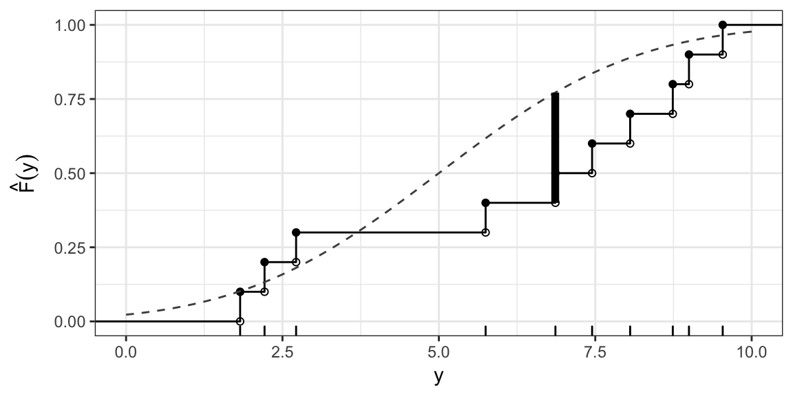
KS test statistic: Normal(5, 6.25)

\(H_0: Y \sim \text{Normal}(5, 6.25)\)

KS test statistic: Example cont.

\(D(F_0) = \sup_{y} \left| \hat{F}(y) - F_0(y) \right| \approx 0.37\) (occurs at \(y\) just less than 6.9)

Reference Distribution?

\[ \sqrt{n} D(F_0) \rightarrow_d K \] where \(K\) is the Kolmogorov Distribution.

Reject \(H_0\) for large values of \(\sqrt{n} D(F_0)\).

In R

ks.test(x = y, y = punif, min = 0, max = 10)

## 
##  One-sample Kolmogorov-Smirnov test
## 
## data:  y
## D = 0.28632, p-value = 0.3209
## alternative hypothesis: two-sided

One sided tests

Lesser alternative: \[ H_A: F < F_0, \text{ i.e. } F(y) < F_0(y) \text{ for all } y \]

Test statistic \[ D^-(H_0) = \sup_y (F_0(y) - \hat{F}(y)) \]

Greater alternative: \[ H_A: F > F_0, \text{ i.e. } F(y) > F_0(y) \text{ for all } y \]

Test statistic \[ D^+(H_0) = \sup_y (\hat{F}(y) - F_0(y) ) \]

One sided tests are hard to interpret

Example based on simulated data. \(H_0: Y \sim N(0, 100)\)

n <- 20
y <- rnorm(n, 0, 1)

For greater alternative: \(H_A: F_Y(y) > \Phi(y; 0, 100)\) where \(\Phi(y; \mu, \sigma^2)\) is the c.d.f of the Normal\((\mu, \sigma)\).

ks.test(y, pnorm, 0, 10, alternative = "greater")

## 
##  One-sample Kolmogorov-Smirnov test
## 
## data:  y
## D^+ = 0.42016, p-value = 0.000513
## alternative hypothesis: the CDF of x lies above the null hypothesis

One sided tests are hard to interpret

For lower alternative: \(H_A: F_Y(y) < \Phi(y; 0, 100)\):

ks.test(y, pnorm, 0, 10, alternative = "less")

## 
##  One-sample Kolmogorov-Smirnov test
## 
## data:  y
## D^- = 0.44858, p-value = 0.0001717
## alternative hypothesis: the CDF of x lies below the null hypothesis

One sided tests

The combination of the two one-sided alternatives, does not cover all the possibilities for which the null hypothesis is false.

This makes it very hard to interpret one-sided KS tests - i.e. don’t do a one-sided test.

Estimating parameters

The KS test should only be used if you can completely specify \(F_0\), the population distribution under the null hypothesis.

You should not estimate parameters from the data then do the test.

Kind of like trying to test \(H_0: \mu = \overline{Y}\), you’ll rarely reject.

Next time…

After midterm: what if distribution is discrete?