Central Limit Theorem ST551 Lecture 6

Central Limit Theorem (CLT)

If the population distribution of a variable $X$ has population mean $\mu$ and (finite) population variance ${\sigma }^2$, then the sampling distribution of the sample mean becomes closer and closer to a Normal distribution as the sample size n increases.

We can write: $$\overline{X}\dot{\sim }N\left(\mu ,\frac{{\sigma }^2}{n}\right)$$ for large values of $n$, where the symbol $\dot{\sim }$ means approximately distributed as.

We already figured out the mean and variance, the CLT adds the shape information

Central Limit Theorem (CLT)

Slightly more formally..

Let $X_1,X_2,\dots ,X_n$ be an i.i.d. sample from some population distribution $F$ with mean $\mu$ and variance ${\sigma }^2<\infty$. Then as the sample size $n\to \infty$ we have

$$\frac{\overline{X}-\mu }{\sigma }{\to }_{D}N\left(0,1\right)$$

Your Turn

Consider the following population distribution.

The following three histograms represent:

1. A sample of size 1000 from the population

2. 1000 sample means of samples of size 10 from the population

3. 1000 sample means of samples of size 100 from the population

Which is which?

How big is big enough?

What value of $n$ is big enough for the approximation to be good enough?

It depends on the population

How big is big enough?

What value of $n$ is big enough for the approximation to be good enough?

It depends on the population

See more in lab…

Your turn

Using the CLT to approximation the sampling distribution

Population: $\sim (\mu =20,{\sigma }^2=4)$
Sample: $n=16$ i.i.d from population
Sample statistic: Sample mean

What is the approximate distribution for $\overline{Y}$?

Applying CLT

Same setup: we have sample of size, $n=16$ from a population with population mean $\mu =20$ and population variance ${\sigma }^2=4$.

What is the probability the sample mean is less than 20.5?

CLT says:

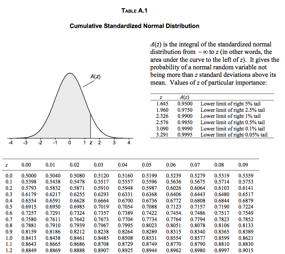
Using a Standard Normal Probability Table

To use a Standard Normal table, we first need to transform our random variable ($\overline{Y}$) to a Standard Normal.

We can convert a probability for $\overline{Y}$ to a standard Normal probability by:

1. Subtracting the mean of $\overline{Y}$ from both sides, then
2. Dividing both sides by the standard deviation of $\overline{Y}$ (square root of the variance)

$$\begin{array}{cc}P(\overline{Y}\le 20.5)& =\end{array}$$

$$\text{where}Z\sim N(0,1)$$

Using a Standard Normal Probability Table

Now look up $z=1.00$ in Standard Normal Table.

$P(\overline{Y}\le 20.5)=0.8413$

Using a Standard Normal Probability Table

What if $z$ is negative?

Standard Normal is symmetric around zero.

$P(Z\le -z)=1-P(Z\le z)$

Density

Density: height of probability density function at x: $f(x;\mu ,\sigma )$

In R: dnorm(x, mean = mu, sd = sigma)

Cumulative Probability

Cumulative Probability: the area under the probability density function to the right of x: $F(x;\mu ,\sigma )$

In R: pnorm(q, mean = mu, sd = sigma)

Area to left?

Quantiles

Quantile: The $p$th quantile is the value $x$, such that the area to the left of $x$ under the density function is $p$. $F^{-1}(p;\mu =0,{\sigma }^2=1)$

qnorm(p, mean = mu, sd = sigma)

What should these return?

qnorm(0, mean = 0, sd = 1)

qnorm(1, mean = 0, sd = 1)

dnorm(-Inf)

dnorm(Inf)

pnorm(Inf)

pnorm(-Inf)

Exercise: Find probability

Return to example: $\mu =20$ ${\sigma }^2=4$, $n=16$

What is $P(\overline{Y}<20.5)$? What is $P(\overline{Y}<21)$

Exercise: Find sample size for specific variance in sample mean

$\mu =20$ ${\sigma }^2=4$.

What should $n$ be so $Var\left(\overline{Y}\right)=0.5$?

Exercise: Find sample size for an interval with desired probability

What should $n$ be, so that $P(19.5<\overline{Y}<20.5)=0.9$?